Transverse Mercator projection
The transverse Mercator map projection is an adaptation of the standard Mercator projection. The transverse version is widely used in national and international mapping systems around the world, including the UTM. When paired with a suitable geodetic datum, the transverse Mercator delivers high accuracy in zones less than a few degrees in east-west extent.
The standard (or Normal) Mercator and the transverse Mercator are two different aspects of the same mathematical construction. Because of the common foundation, the transverse Mercator inherits many traits from the normal Mercator.
- Both projections are cylindrical: for the Normal Mercator, the axis of the cylinder coincides with the polar axis and the line of tangency with the equator. For the transverse Mercator, the axis of the cylinder lies in the equatorial plane, and the line of tangency is any chosen meridian, thereby designated the central meridian.
- Both projections may be modified to secant forms, which means the scale has been reduced so that the cylinder slices through the model globe.
- Both exist in spherical and ellipsoidal versions.
- Both projections are conformal, so that the point scale is independent of direction and local shapes are well preserved;
- Both projections have constant scale the line of tangency (the equator for the normal Mercator and the central meridian for the transverse).
Since the central meridian of the transverse Mercator can be chosen at will, it may be used to construct highly accurate maps (of narrow width) anywhere on the globe. The secant, ellipsoidal form of the transverse Mercator is the most widely applied of all projections for accurate large scale maps.
Contents |
General features of the spherical transverse Mercator
In constructing a map on any projection, a sphere is normally chosen to model the earth when the extent of the mapped region exceeds a few hundred kilometers in length in both dimensions. For maps of smaller regions, an ellipsoidal model must be chosen if greater accuracy is required; see next section. The spherical form of the transverse Mercator projection was one of the seven 'new' projections presented, in 1772, by Johann Heinrich Lambert[1][2] (also available in a modern English translation).[3] Lambert did not name his projections; the name transverse Mercator dates from the second half of the nineteenth century.[4] The principal properties of the transverse projection are here presented in comparison with the properties of the normal projection.
A comparison of normal and transverse projections on the sphere
| Normal Mercator | Transverse Mercator | |||
|---|---|---|---|---|
| • | The central meridian projects to the straight line x = 0. Other meridians project to straight lines with x constant. | • | The central meridian projects to the straight line x = 0. Meridians 90 degrees east and west of the central meridian project to lines of constant y through the projected poles. All other meridians project to complicated curves. | |
| • | The equator projects to the straight line y = 0 and parallel circles project to straight lines of constant y. | • | The equator projects to the straight line y = 0 but all other parallels are complicated closed curves. | |
| • | Projected meridians and parallels intersect at right angles. | • | Projected meridians and parallels intersect at right angles. | |
| • | The projection is unbounded in the y direction. The poles lie at infinity. | • | The projection is unbounded in the x direction. The points on the equator at ninety degrees from the central meridian are projected to infinity. | |
| • | The projection is conformal. The shapes of small elements are well preserved. | • | The projection is conformal. The shapes of small elements are well preserved. | |
| • | Distortion increases with y. The projection is not suited for world maps. Distortion is small near the equator and the projection (particularly in its ellipsoidal form) is suitable for accurate mapping of equatorial regions. | • | Distortion increases with x. The projection is not suited for world maps. Distortion is small near the central meridian and the projection (particularly in its ellipsoidal form) is suitable for accurate mapping of narrow regions. | |
| • | Greenland is almost as large as Africa; the actual area is about one thirteenth that of Africa. | • | Greenland and Africa are both near to the central meridian; their shapes are good and the ratio of the areas is a good approximation to actual values. | |
| • | The point scale factor is independent of direction. It is a function of y on the projection. (On the sphere it depends on latitude only.) The scale is true on the equator. | • | The point scale factor is independent of direction. It is a function of x on the projection. (On the sphere it depends on both latitude and longitude.) The scale is true on the central meridian. | |
| • | The projection is reasonably accurate near the equator. Scale at an angular distance of 5° (in latitude) away from the equator is less than 0.4% greater than scale at the equator, and is about 1.54% greater at an angular distance of 10°. | • | The projection is reasonably accurate near the central meridian. Scale at an angular distance of 5° (in longitude) away from the central meridian is less than 0.4% greater than scale at the central meridian, and is about 1.54% at an angular distance of 10°. | |
| • | In the secant version the scale is reduced on the equator and it is true on two lines parallel to the projected equator (and corresponding to two parallel circles on the sphere). | • | In the secant version the scale is reduced on the central meridian and it is true on two lines parallel to the projected central meridian. | |
| • | Convergence (the angle between projected meridians and grid lines with x constant) is identically zero. Grid north and true north coincide. | • | Convergence is zero on the equator and non-zero everywhere else. It increases as the poles are approached. Grid north and true north do not coincide. | |
| • | Rhumb lines (of constant compass bearing on the sphere) project to straight lines. | • | Rhumb lines project to complex curves. |
General features of the ellipsoidal transverse Mercator
The ellipsoidal form of the transverse Mercator projection was developed by Carl Friedrich Gauss in 1825[5] and further analysed by Johann Heinrich Louis Krüger in 1912.[6] The projection is known by several names: Gauss Conformal or Gauss-Krüger in Europe; the transverse Mercator in the US; or Gauss-Krüger transverse Mercator generally. The projection is conformal with a constant scale on the central meridian. (There are other conformal generalisations of the transverse Mercator from the sphere to the ellipsoid but only Gauss-Krüger has a constant scale on the central meridian.) Throughout the twentieth century the Gauss-Krüger transverse Mercator was adopted, in one form or another, by many nations (and international bodies);[7] in addition it provides the basis for the Universal Transverse Mercator series of projections. The Gauss-Krüger projection is now the most widely used projection in accurate large scale mapping.
The projection, as developed by Gauss and Krüger, was expressed in terms of low order power series which were assumed to diverge in the east-west direction, exactly as in the spherical version. This was proved to be untrue by British cartographer E.H. Thompson, whose unpublished exact (closed form) version of the projection, reported by L.P. Lee in 1976,[8] showed that the ellipsoidal projection is finite (below). This is the most striking difference between the spherical and ellipsoidal versions of the transverse Mercator projection: Gauss-Krüger gives a reasonable projection of the whole ellipsoid to the plane, although its principal application is to accurate large scale mapping "close" to the central meridian.
Features of the projection are as follows:
-
- Near the central meridian (Greenwich in the above example) the projection has low distortion and the shapes of Africa, western Europe, Britain, Greenland, Antarctica compare favourably with a globe.
- The central regions of the transverse projections on sphere and ellipsoid are indistinguishable on the small scale projections shown here.
- The meridians at 90° east and west of the chosen central meridian project to horizontal lines through the poles. The more distant hemisphere is projected above the north pole and below the south pole.
- The equator bisects Africa, crosses South America and then continues onto the complete outer boundary of the projection; the top and bottom edges and the right and left edges must be identified (i.e. they represent the same lines on the globe). (Indonesia is bisected).
- Distortion increases towards the right and left boundaries of the projection but it does not increase to infinity. Note the Galapagos Islands where the 90° west meridian meets the equator at bottom left.
- The map is conformal. Lines intersecting at any specified angle on the ellipsoid project into lines intersecting at the same angle on the projection. In particular parallels and meridians intersect at 90°.
- The point scale factor is independent of direction at any point so that the shape of a small region is reasonably well preserved. The necessary condition is that the magnitude of scale factor must not vary too much over the region concerned. Note that while South America is distorted greatly the island of Ceylon is small enough to be reasonably shaped although it is far from the central meridian.
- The choice of central meridian greatly affects the appearance of the projection. If 90°W is chosen then the whole of the Americas is reasonable. If 145°E is chosen the Far East is good and Australia is oriented with north up.
In most applications the Gauss–Krüger is applied to a narrow strip near the central meridians where the differences between the spherical and ellipsoidal versions are small, but nevertheless important in accurate mapping. Direct series for scale, convergence and distortion are functions of eccentricity and both latitude and longitude on the ellipsoid: inverse series are functions of eccentricity and both x and y on the projection. In the secant version the lines of true scale on the projection are no longer parallel to central meridian; they curve slightly. The convergence angle between projected meridians and the x constant grid lines is no longer zero (except on the equator) so that a grid bearing must be corrected to obtain a true compass bearing. The difference is small, but not negligible, particularly at high latitudes.
Implementations of the Gauss–Krüger projection
In his 1912[6] paper Krüger presented two distinct solutions, distinguished here by the expansion parameter:
- Krüger–n (paragraphs 5 to 8). Formulae for the direct projection, giving the coordinates x and y, are fourth order expansions in terms of the third flattening, n (the ratio of the difference and sum of the major and minor axes of the ellipsoid). The coefficients are expressed in terms of latitude (φ), longitude (λ), major axis (a) and eccentricity (e). The inverse formulae for φ and λ are also fourth order expansions in n but with coefficients expressed in terms of x, y, a and e. (See Transverse Mercator: flattening series)
- Krüger–λ (paragraphs 13 and 14). Formulae giving the projection coordinates x and y are expansions (of orders 5 and 4 respectively) in terms of the longitude λ, expressed in radians: the coefficients are expressed in terms of φ, a and e. The inverse projection for φ and λ are sixth order expansions in terms of the ratio x/a, with coefficients expressed in terms of y, a and e. (See Transverse Mercator: Redfearn series)
The Krüger–λ series were the first to be implemented, possibly because they were much easier to evaluate on the hand calculators of the mid twentieth century.
- Lee–Redfearn–OSGB. In 1946 L.P.Lee[9] confirmed the λ expansions of Krüger and proposed their adoption by the OSGB[10] but Redfearn (1948)[11] pointed out that they were not accurate because of (a) the relatively high latitudes of Great Britain and (b) the great width of the area mapped, over 10 degrees of longitude. Redfearn extended the series to eighth order and examined which terms were necessary to attain an accuracy of 1mm (ground measurement). The Redfearn series are still the basis of the OSGB map projections.[10]
- Thomas–UTM The λ expansions of Krüger were also confirmed by Paul Thomas in 1952:[12] they are readily available in Snyder.[13] His projection formulae, completely equivalent to those presented by Redfearn, were adopted by the United States Defence Mapping Agency as the basis for the UTM.[14] They are also incorporated into the Geotrans[15] coordinate converter made available by the United States National Geospatial-Intelligence Agency [3].
- Other countries. The Redfearn series are the basis for geodetic mapping in many countries: Australia, Germany, Canada, South Africa to name but a few. (A list is given in Appendix A.1 of Stuifbergen 2009.)[16]
- Many variants of the Redfearn series have been proposed but only those adopted by national cartographic agencies are of importance. For an example of modifications which do not have this status see Transverse Mercator: Bowring series). All such modifications have been eclipsed by the power of modern computers and the development of high order n-series outlined below. The precise Redfearn series, although of low order, cannot be disregarded as they are still enshrined in the quasi-legal definitions of OSGB and UTM etc.
The Krüger–n series are described on the page [[Transverse Mercator: series in n (third flattening)]]. They have been implemented (to fourth order in n) by the following nations.
Higher order versions of the Krüger–n series have been implemented to seventh order by Ensager and Poder[20] and to tenth order by Kawase.[21] Apart from a series expansion for the transformation between latitude and conformal latitude, Karney has implemented the series to thirtieth order.[22]
Exact Gauss-Krüger and accuracy of the truncated series
The exact solution of E. H. Thompson, described by L.P. Lee,[8] is summarized on the page Transverse Mercator: exact solution. It is constructed in terms of elliptic functions (defined in chapters 19 and 22 of the NIST[23] handbook) which can be calculated to arbitrary accuracy using algebraic computing systems such as Maxima.[24] Such an implementation of the exact solution is described by Karney (2011).[22]
The exact solution is a valuable tool in assessing the accuracy of the truncated n and λ series. For example, the original 1912 Krüger–n series compares very favourably with the exact values: they differ by less than 0.31 μm within 1000 km of the central meridian and by less than 1 mm out to 6000 km. On the other hand the difference of the Redfearn series used by Geotrans and the exact solution is less than 1 mm out to a longitude difference of 3 degrees, corresponding to a distance of 334 km from the central meridian at the equator but a mere 35 km at the northern limit of an UTM zone. Thus the Krüger–n series are very much better than the Redfearn λ series.
The Redfearn series become much worse as the zone widens. Karney discusses Greenland as an instructive example. The long thin landmass is centred on 42W and, at its broadest point, is no more than 750 km from that meridian while the span in longitude reaches almost 50 degrees. Krüger–n is accurate to within 1mm but the Redfearn version of the Krüger–λ series has a maximum error of 1 kilometre.
Karney's own 8th order (in n) series is accurate to 5 nm within 3900 km of the central meridian.
Formulae for the spherical transverse Mercator
Spherical normal Mercator revisited
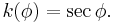
The normal cylindrical projections are described in relation to a cylinder tangential at the equator with axis along the polar axis of the sphere. The cylindrical projections are constructed so that all points on a meridian are projected to points with  and
and  a prescribed function of
  . For a tangent Normal Mercator projection the (unique) formulae which guarantee conformality are[25]:
![x = a\lambda\,,\qquad
y = a\ln \bigg[\tan \bigg(\frac{\pi}{4} %2B \frac{\phi}{2} \bigg)\bigg]
= \frac{a}{2}\ln\left[\frac{1%2B\sin\phi}{1-\sin\phi}\right].](/2012-wikipedia_en_all_nopic_01_2012/I/4b8ee36622b776a0ee01a4c13905a125.png)
Conformality implies that the point scale,  , is independent of direction: it is a function of latitude only:
For the secant version of the projection there is a factor of  on the right hand side of all these equations: this ensures that the scale is equal to on the equator.
Normal and transverse graticules
The figure on the left shows how a transverse cylinder is related to the conventional graticule on the sphere. It is tangential to some arbitrarily chosen meridian and its axis is perpendicular to that of the sphere. The  and axes defined on the figure are related to the equator and central meridian exactly as they are for the normal projection. In the figure on the right a rotated graticule is related to the transverse cylinder in the same way that the normal cylinder is related to the standard graticule. The 'equator', 'poles' (E and W) and 'meridians' of the rotated graticule are identified with the chosen central meridian, points on the equator 90 degrees east and west of the central meridian, and great circles through those points.
The position of an arbitrary point  on the standard graticule can also be identified in terms of angles on the rotated graticule:
  (angle M'CP) is an effective latitude and
  (angle M'CO) becomes an effective longitude. (The minus sign is necessary so that
  are related to the rotated graticule in the same way that are related to the standard graticule). The Cartesian
  axes are related to the rotated graticule in the same way that the axes
  axes are related to the standard graticule.
The tangent transverse Mercator projection defines the coordinates in terms of and by the transformation formulae of the tangent Normal Mercator projection:
![x' = -a\lambda'\,\qquad
y' = \frac{a}{2}
\ln\left[\frac{1%2B\sin\phi'}{1-\sin\phi'}\right].](/2012-wikipedia_en_all_nopic_01_2012/I/58d0a73c1ffe2fca364777fcc305b795.png)
This transformation projects the central meridian to a straight line of finite length and at the same time projects the great circles through E and W (which include the equator) to infinite straight lines perpendicular to the central meridian. The true parallels and meridians (other than equator and central meridian) have no simple relation to the rotated graticule and they project to complicated curves.
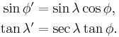
The relation between the graticules
The angles of the two graticules are related by using spherical trigonometry on the spherical triangle NM'P defined by the true meridian through the origin, OM'N, the true meridian through an arbitrary point, MPN, and the great circle WM'PE. The results are[25]:
Direct transformation formulae
The direct formulae giving the Cartesian coordinates follow immediately from the above. Setting  and
and  (and restoring factors of to accommodate secant versions)
![\begin{align}
x(\lambda,\phi)&= \frac{1}{2}k_0a
\ln\left[
\frac{1%2B\sin\lambda\cos\phi}
{1-\sin\lambda\cos\phi}\right],\\
y(\lambda,\phi)&= k_0 a\arctan\left[\sec\lambda\tan\phi\right],
\end{align}](/2012-wikipedia_en_all_nopic_01_2012/I/426ed5d830c57d6a3b98155e2ea22698.png)
The above expressions are given in Lambert[1] and also (without derivations) in Snyder,[13] Maling[26] and online[25] (with full details).
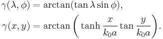
Inverse transformation formulae
Inverting the above equations gives
![\begin{align}
\lambda(x,y)&
= \arctan\bigg[ \sinh\frac{x}{k_0a}
\sec\frac{y}{k_0a} \bigg],
\\[1ex]
\phi(x,y)&= \arcsin\bigg[ \mbox{sech}\;\frac{x}{k_0a}
\sin\frac{y}{k_0a} \bigg].
\end{align}](/2012-wikipedia_en_all_nopic_01_2012/I/a42bf3e742eac334369642321f52b071.png)
Point scale
In terms of the coordinates with respect to the rotated graticule the point scale factor is given by  : this may be expressed either in terms of the geographical coordinates or in terms of the projection coordinates:
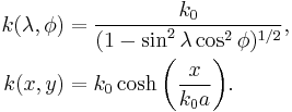
The second expression shows that the scale factor is simply a function of the distance from the central meridian of the projection. A typical value of the scale factor is  so that
  when is approximately 180 km. When is approximately 255 km and
  : the scale factor is within 0.04% of unity over a strip of about 510 km wide.
Convergence
The convergence angle  at a point on the projection is defined by the angle measured from the projected meridian, which defines true north, to a grid line of constant x, defining grid north. Therefore is positive in the quadrant north of the equator and east of the central meridian and also in the quadrant south of the equator and west of the central meridian. The convergence must be added to a grid bearing to obtain a compass bearing from true north. For the secant transverse Mercator the convergence may be expressed[25] either in terms of the geographical coordinates or in terms of the projection coordinates:
Formulae for the ellipsoidal transverse Mercator
- The details of actual implementations of the Gauss-Kruger series in longitude may be found at:
Transverse Mercator: Redfearn series
- The details of actual implementations of the Gauss-Kruger series in n (third flattening) may be found at:
Transverse Mercator: flattening series Page in preparation.
- The details of actual implementations of the exact (closed form) transverse Mercator projection may be found at:
Transverse Mercator: exact solution Page in preparation.
- An example of how the fourth order Redfearn series may be implemented by concise formulae may be found at:
Transverse Mercator: Bowring series
See also
- Jordan Transverse Mercator
- Mercator projection
- Map projection
- Scale (map)
- Universal Transverse Mercator coordinate system
References
- ^ a b Lambert, Johann Heinrich. 1772. Ammerkungen und Zusatze zurder Land und Himmelscharten Entwerfung. In Beyträge zum Gebrauche der Mathematik und deren Anwendung, part 3, section 6)
- ^ Albert Wangerin (Editor), 1894. Ostwald's Klassiker der exacten Wissenschaften (54). Published by Wilhelm Engelmann. This is Lambert's paper with additional comments by the editor. Available at the University of Michigan Historical Math Library.
- ^ Tobler, Waldo R, Notes and Comments on the Composition of Terrestrial and Celestial Maps, 1972. University of Michigan Press
- ^ Snyder, John P. (1993). Flattening the Earth: Two Thousand Years of Map Projections. University of Chicago Press. p. 82. ISBN 0-226-76747-7. This is an excellent survey of virtually all known projections from antiquity to 1993.
- ^ Gauss, Karl Friedrich, 1825. "Allgemeine Auflösung der Aufgabe: die Theile einer gegebnen Fläche auf einer andern gegebnen Fläche so abzubilden, daß die Abbildung dem Abgebildeten in den kleinsten Theilen ähnlich wird" Preisarbeit der Kopenhagener Akademie 1822. Schumacher Astronomische Abhandlungen, Altona, no. 3, p. 5–30. [Reprinted, 1894, Ostwald’s Klassiker der Exakten Wissenschaften, no. 55: Leipzig, Wilhelm Engelmann, p. 57–81, with editing by Albert Wangerin, pp. 97–101. Also in Herausgegeben von der Gesellschaft der Wissenschaften zu Göttingen in Kommission bei Julius Springer in Berlin, 1929, v. 12, pp. 1–9.]
- ^ a b Krüger, L. (1912). Konforme Abbildung des Erdellipsoids in der Ebene. Royal Prussian Geodetic Institute, New Series 52.
- ^ "Short Proceedings of the 1st European Workshop on Reference Grids, Ispra, 27–29 October 2003". European Environment Agency. 2004-06-14. p. 6. http://eusoils.jrc.ec.europa.eu/Projects/Alpsis/Docs/ref_grid_sh_proc_draft.pdf. Retrieved 2009-08-27.The EEA recommends the transverse Mercator for conformal pan-European mapping at scales larger than 1:500,000
- ^ a b Lee, L.P. (1976). Conformal Projections Based on Elliptic Functions. Supplement No. 1 to Canadian Cartographer, Vol 13. (Designated as Monograph 16). Toronto: Department of Geography, York University. A report of unpublished analytic formulae involving incomplete elliptic integrals obtained by E.H. Thompson in 1945. The article may be purchased from University of Toronto [1]. At the present time (2010) it is necessary to purchase several units in order to obtain the relevant pages: pp 1–14, 92–101 and 107–114.
- ^ Lee L P, (1946). Survey Review, Volume 8 (Part 58), pp 142–152. The transverse Mercator projection of the spheroid. (Errata and comments in Volume 8 (Part 61), pp 277–278.
- ^ a b A guide to coordinate systems in Great Britain. This is available as a pdf document at [2]
- ^ Redfearn, J C B (1948). Survey Review, Volume 9 (Part 69), pp 318–322, Transverse Mercator formulae.
- ^ Thomas, Paul D (1952). Conformal Projections in Geodesy and Cartography. Washington: U.S. Coast and Geodetic Survey Special Publication 251.
- ^ a b Snyder, John P. (1987). Map Projections – A Working Manual. U.S. Geological Survey Professional Paper 1395. United States Government Printing Office, Washington, D.C..This paper can be downloaded from USGS pages. It gives full details of most projections, together with interesting introductory sections, but it does not derive any of the projections from first principles.
- ^ J. W. Hager, J.F. Behensky, and B.W. Drew, 1989, The universal grids: Universal Transverse Mercator (UTM) and Universal Polar Stereographic (UPS), Technical Report TM 8358.2, Defense Mapping Agency, URL http://earth-info.nga.mil/GandG/ publications/tm8358.2/TM8358 2.pdf.
- ^ Geotrans, 2010, Geographic translator, version 3.0, URL http://earth-info.nga.mil/GandG/geotrans/
- ^ N. Stuifbergen, 2009, Wide zone transverse Mercator projection, Technical Report 262, Canadian Hydrographic Service, URL http://www.dfo-mpo.gc.ca/Library/337182.pdf.
- ^ [www.ign.fr/DISPLAY/000/526/702/5267021/NTG_76.pdf]
- ^ R. Kuittinen, T. Sarjakoski, M. Ollikainen, M. Poutanen, R. Nuuros, P. T¨atil¨a, J. Peltola, R. Ruotsalainen, and M. Ollikainen, 2006, ETRS89—j¨arjestelm¨a¨an liittyv¨at karttaprojektiot, tasokoordinaatistot ja karttalehtijako, Technical Report JHS 154, Finnish Geodetic Institute, Appendix 1, Projektiokaavart, URL http://docs.jhs-suositukset.fi/jhs-suositukset/JHS154/JHS154 liite1.pdf.
- ^ http://www.lantmateriet.se/upload/filer/kartor/geodesi_gps_och_detaljmatning/geodesi/Formelsamling/Gauss_Conformal_Projection.pdf
- ^ K. E. Engsager and K. Poder, 2007, A highly accurate world wide algorithm for the transverse Mercator mapping (almost), in Proc. XXIII Intl. Cartographic Conf. (ICC2007), Moscow, p. 2.1.2.
- ^ Kawase, K. (2011): A General Formula for Calculating Meridian Arc Length and its Application to Coordinate Conversion in the Gauss-Krüger Projection, Bulletin of the Geospatial Information Authority of Japan, 59, pp 1–13
- ^ a b C. F. F. Karney (2011), Transverse Mercator with an accuracy of a few nanometers, J. Geodesy 85(8), 475-485 (2011); preprint of paper and C++ implementation of algorithms are available at tm.html.
- ^ F. W.J. Olver, D.W. Lozier, R.F. Boisvert, and C.W. Clark, editors,2010, NIST Handbook of Mathematical Functions (Cambridge University Press), available online at URL http://dlmf.nist.gov.
- ^ Maxima, 2009, A computer algebra system, version 5.20.1, URL http://maxima.sf.net.
- ^ a b c d The Mercator Projections Detailed derivations of all formulae quoted in this article
- ^ Maling, Derek Hylton (1992). Coordinate Systems and Map Projections (second ed.). Pergamon Press. ISBN 0-08-037033-3..
External links
- The projections used to illustrate this article were prepared using Geocart which is available from http://www.mapthematics.com